part of Course 193 How Neural Networks Work

We’re going to try and build a comfortable intuition, a solid understanding, of what backpropagation is and how it works.

This is part of the End to End Machine Learning school library. You can find a lot more tutorials and courses at e2eml.school.

Backpropagation from scratch

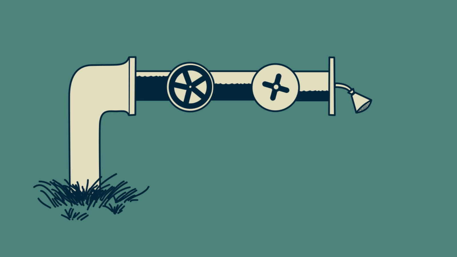
We’re going to use Backpropagation to take the perfect shower. Imagine your shower head is finicky. If you don’t get the flow rate just right, you get a terrible shower. Too little flow and it feels like it’s dripping. Too much flow and it feels like a firehose. There’s a very narrow range where it’s comfortable.

You have two valves that adjust the water flow rate: the shower handle, and the main valve for the house. By adjusting either one of them, you can adjust the flow rate through the shower head, making it faster or slower. We’re going to use backpropagation to get them adjusted just right.

The shower flow rate depends on the setting of both of these valves. We care about how sensitive it is to both valve settings. If we turn the shower handle a quarter turn, does the shower flow rate change a lot or a little? Is it sensitive to the shower handle position or not very?

Sensitivity

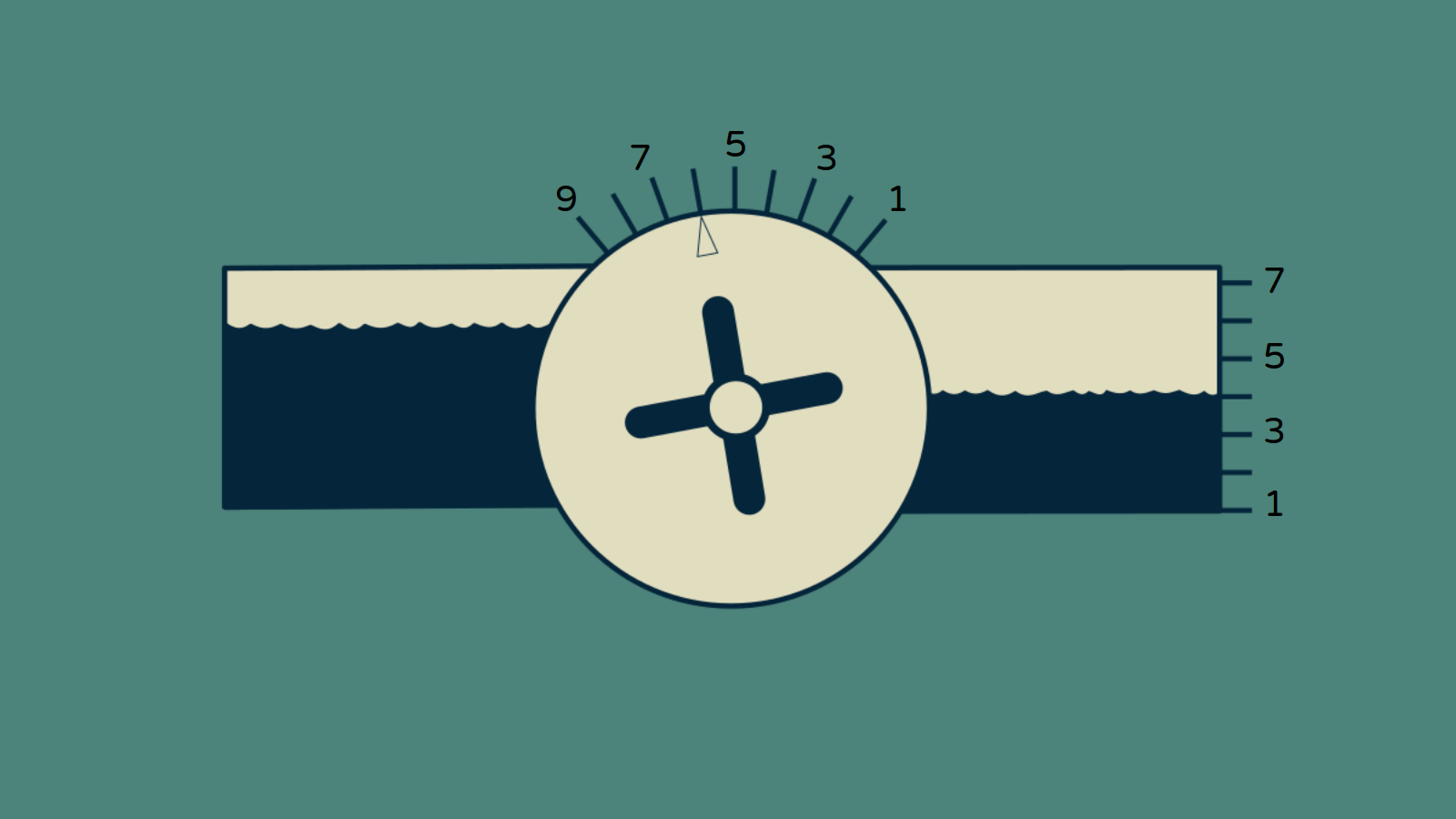
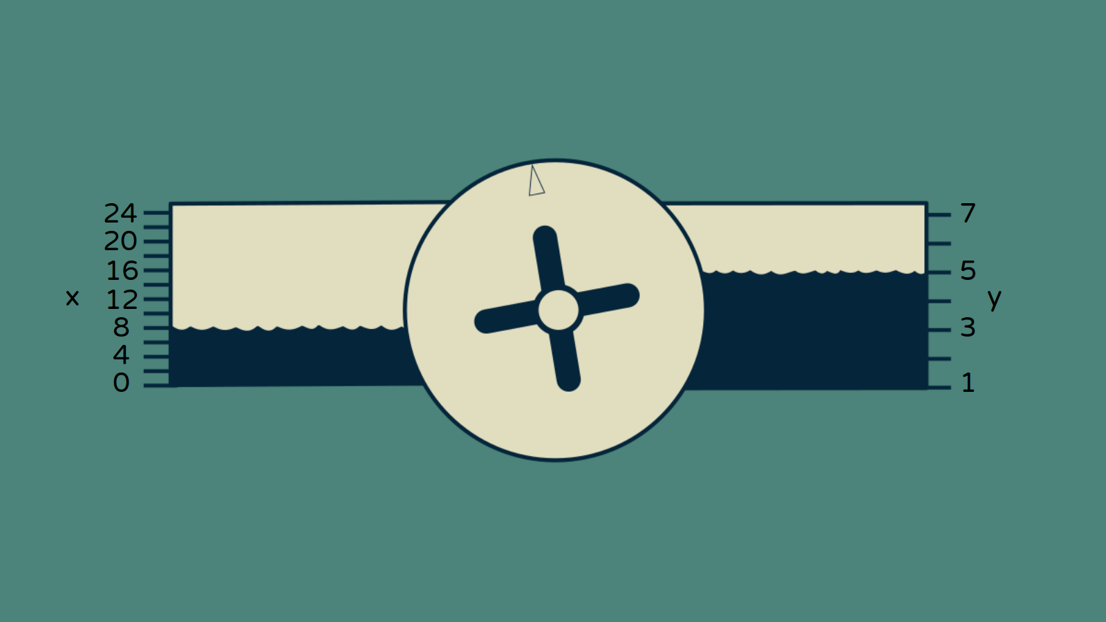
We can put a number on sensitivity. First we start by measuring the shower handle position. Let’s assume that positions on the shower handle are numbered 1 through 10. If we adjust it from a 2 to 3, that’s a change of one unit.

We can also measure the flow rate at the showerhead in units of cubic feet per minute. If the flow rate changes from 4 to 5 cubic feet per minute, that’s a change of one unit.

We can adjust the shower handle by a certain amount and observe how much the shower flow rate changes. Let’s say we change the shower handle position from 4 to 8. That is a change of four units. Then we notice that the shower flow rate changes from 3 to 5 cubic feet per minute. That’s a change of two units. By dividing the change in the shower flow rate by the change in the handle position, we can find the sensitivity of shower flow rate to handle position. In this case it is (5-3) / (8-4), or 2 / 4, or one half. Sensitivity is a way of quantifying how much the shower flow rate will change if we adjust the shower handle up by one position. For each unit increase in shower handle position, we can expect the flow rate to increase by on half unit.

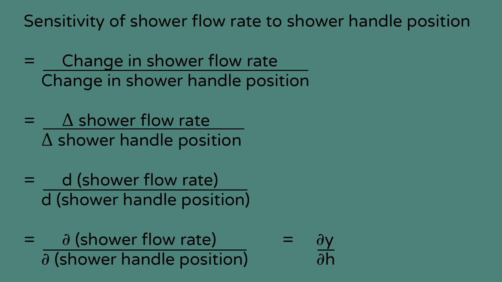
Saying it in math

The terminology quickly becomes awkward. Luckily math helps us out here. Sensitivity is change in one thing per a one unit change in another thing, change in shower flow rate per one unit change in the shower handle position for instance. This can be written Δ shower flow rate divided by Δ shower handle setting. Δ, the capital Greek d, is a common way to indicate a change in a variable. Or, if we want to talk about the relationship between very small changes in both of these items, we can use the calculus notation of d(showerhead flow rate) divided by d(shower handle position). This is a way to express the derivative of the shower flow rate with respect to the shower handle setting. Since the flow rate is actually sensitive to two different things, the shower handle setting and the house flow rate going into the shower handle, it is most accurate to write sensitivity as ∂(showerhead flow rate) divided by ∂ (shower handle position). This means the partial derivative of shower flow rate with respect to shower handle setting. But they all mean the same thing. Conceptually we’re just expressing the sensitivity of the thing on top to changes of the thing on the bottom. Because they are the most technically correct and because they look cool, we'll use the curly D’s: ∂.

To make our conversation even a little more concise, we can give things shorter names. We'll call the shower flow rate y and the shower handle position h. We can call the flow rate in the house x, and the pressure in the water main w, and the position of the main valve m. Now we can use these short names to call the sensitivity of the shower flow rate to the shower handle position ∂y/∂h.

Working backward

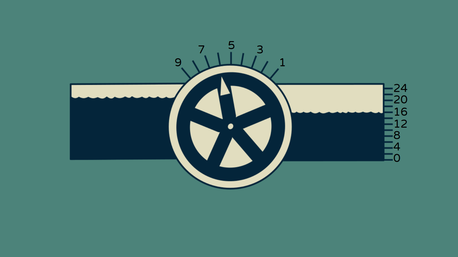
We can also find the sensitivity for the main house valve. We can measure both the main valve position m and the resulting house flow rate x and we can observe how the latter changes when we adjust the former. By dividing our change in x by our change in m, we can calculate the sensitivity of house flow rate to main valve setting, ∂x/∂h.

The output flow rate of the showerhead y depends both on the shower handle setting h and the house flow rate flowing into the shower handle x. We can put a number on this sensitivity too. Adjusting the main valve m changes the house flow rate x which indirectly affects the shower flow rate y. By measuring the change in the house flow rate x and the corresponding change in the flow rate through the showerhead y, we can find the sensitivity of the shower flow rate to increases in the house flow rate, ∂y/∂x.

The Chain Rule

So now we have a few different sensitivities, ∂y/∂h, ∂y/∂x, and ∂x/∂m. This is a solid start. This is exactly what we need to start calculating what adjustments we need to make.

One thing that jumps out is that we don’t actually know the sensitivity of the shower flow rate with respect to the main valve. We don’t know ∂y/∂m. However, with a little bit of puzzling we can figure it out. Imagine that we had measured ∂x/∂m to be two. For every unit change in main valve position, the house flow rate increases by two. Also assume that we had measured ∂y/∂x to be 1/4. For every unit change in house flow rate, the showerhead flow rate increases by 1/4 unit. Now, we can play out what would happen to the showerhead flow rate if we increase the main valve position by one unit. ∂x/∂m says the house flow rate would go up by two. And since we know that every unit of house flow rate increases the showerflow rate by 1/4, we can multiply the two together to get the net result. 2×1/4 equals 1/2. A unit change in main valve position gives an increase of showerhead flow rate of half a unit.

This example is pretty straightforward to think about, so the power of what we just did may not be immediately obvious. We chained together two sensitivities by multiplying them. ∂y/∂m = ∂y/∂x × ∂x/∂m. Calculus tells us that this doesn’t just work for our example here, but it works all the time everywhere for any chain of sensitivities, no matter how long. Not surprisingly, it’s called the Chain Rule. And it will be the secret to our success in backpropagation.

Now we are in a good position to start making adjustments. We have the sensitivity of the thing we care about, the shower flow rate, with respect to the two things that we can change, the main valve setting and the shower handle setting. Armed with these, we are ready to get our shower going.

How far from ideal is the shower?

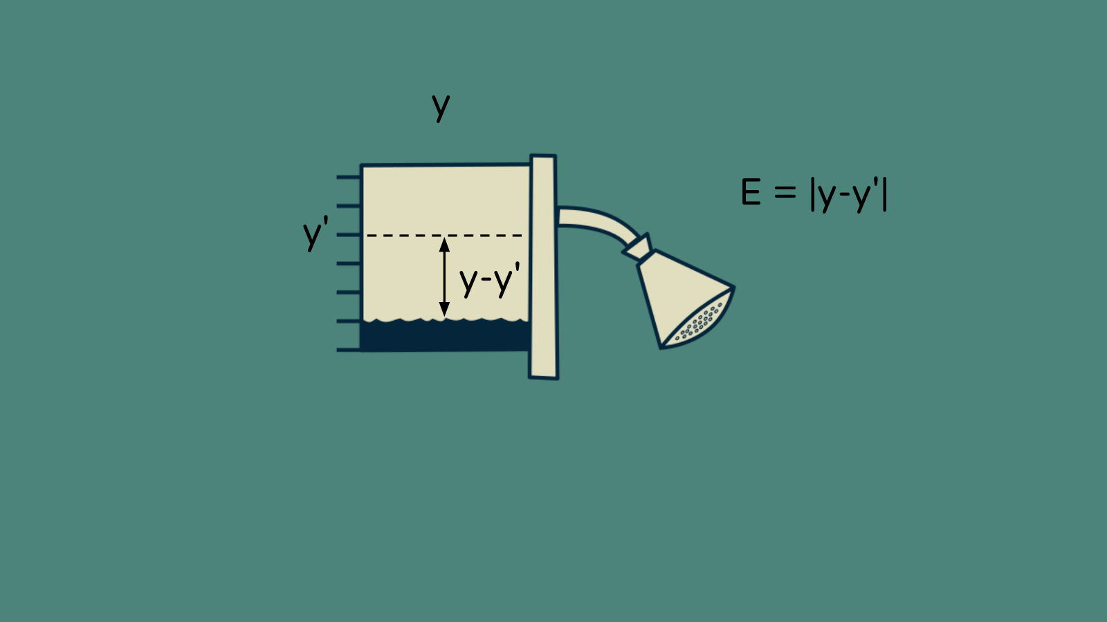
Let’s say that our ideal shower flow rate is a special value of y, which we’ll call y'. We can calculate our deviation, how far away from this ideal value we are, by taking y - y'. To express our unhappiness with the current state of the water flow, we can use how far away it is from the ideal: the absolute value of y - y’ or |y - y'|. We'll call this E, our error, and we would like for it to be zero. Our goal will be to adjust our valves m and h to make our shower flow rate perfect, drive y to be y prime, and make and E go to zero.

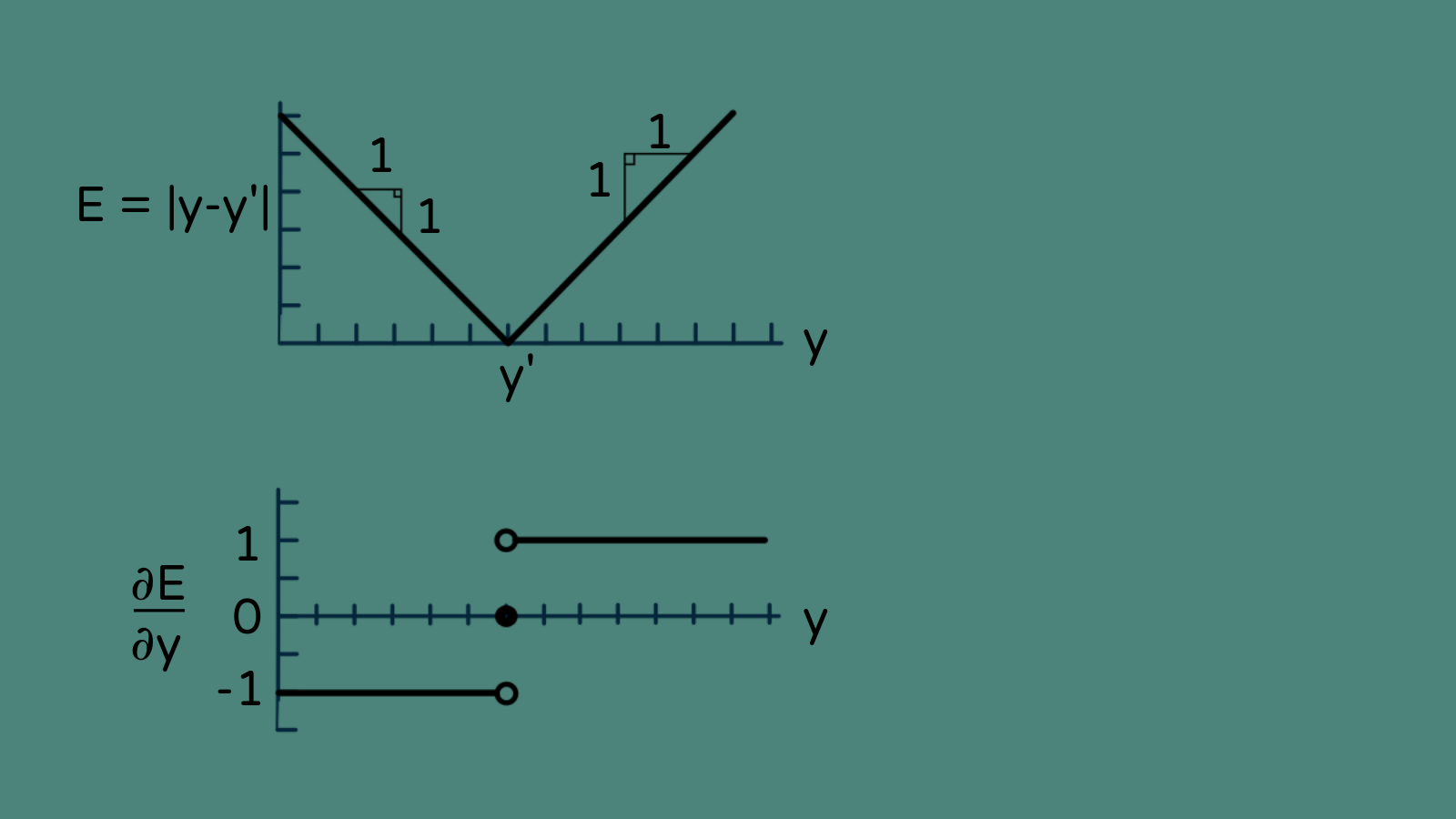
Since we’re in the business of calculating sensitivities, we can also find the sensitivity of E to changes in our shower flow rate. The derivative of an absolute value is straightforward:

∂E/∂y = 1 if y is greater than y' and it’s -1 if it’s less than y'. It’s not actually defined at y = y', but we can just declare it to be zero.

Now we can chain this with our other sensitivities to find the sensitivity of the error to our two valve positions.

How to split the adjustment between valves?

Now we have one thing we want to change, the error, and two ways to change it. How do we go about it? Do we try to get away with turning just one valve? Split the difference between the two? There are any number of ways to get the results we want. Which do we choose? This is where backpropagation comes in.

The recipe that backpropagation uses to choose how much to adjust each valve is to weight the adjustments by the sensitivity. Is the shower flow rate error twice as sensitive to the main valve position m as it is to the shower handle position h? Then adjust the main valve twice as much as the shower handle. The benefits of focusing adjustments on the most sensitive valve aren’t obvious in this simple example, but in a more complex situation (imagine hundreds of showers connected through thousands of pipes to millions of valves) it helps encourage specialization. It leads to a few valves and pipes being closely tied to a single shower.

How much should each valve be adjusted?

Knowing the sensitivities and the size of the change that we hope to make, it’s tempting to try to get to the perfect shower flow in one go, touching each of the valves just once.

There are three good reasons not to do this.

The first reason is that we may not be able to get to a zero error. It’s possible that the water main has low pressure and even with both valves wide open our shower would be slower than we want. This is the case much more often than not. Depending on how our error E is defined, the best we can do might be some number other than zero. We don’t know what that best value is, so we’re kind of hunting in the dark for it.

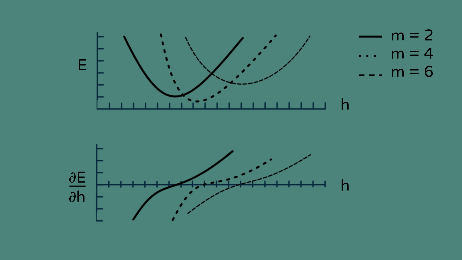
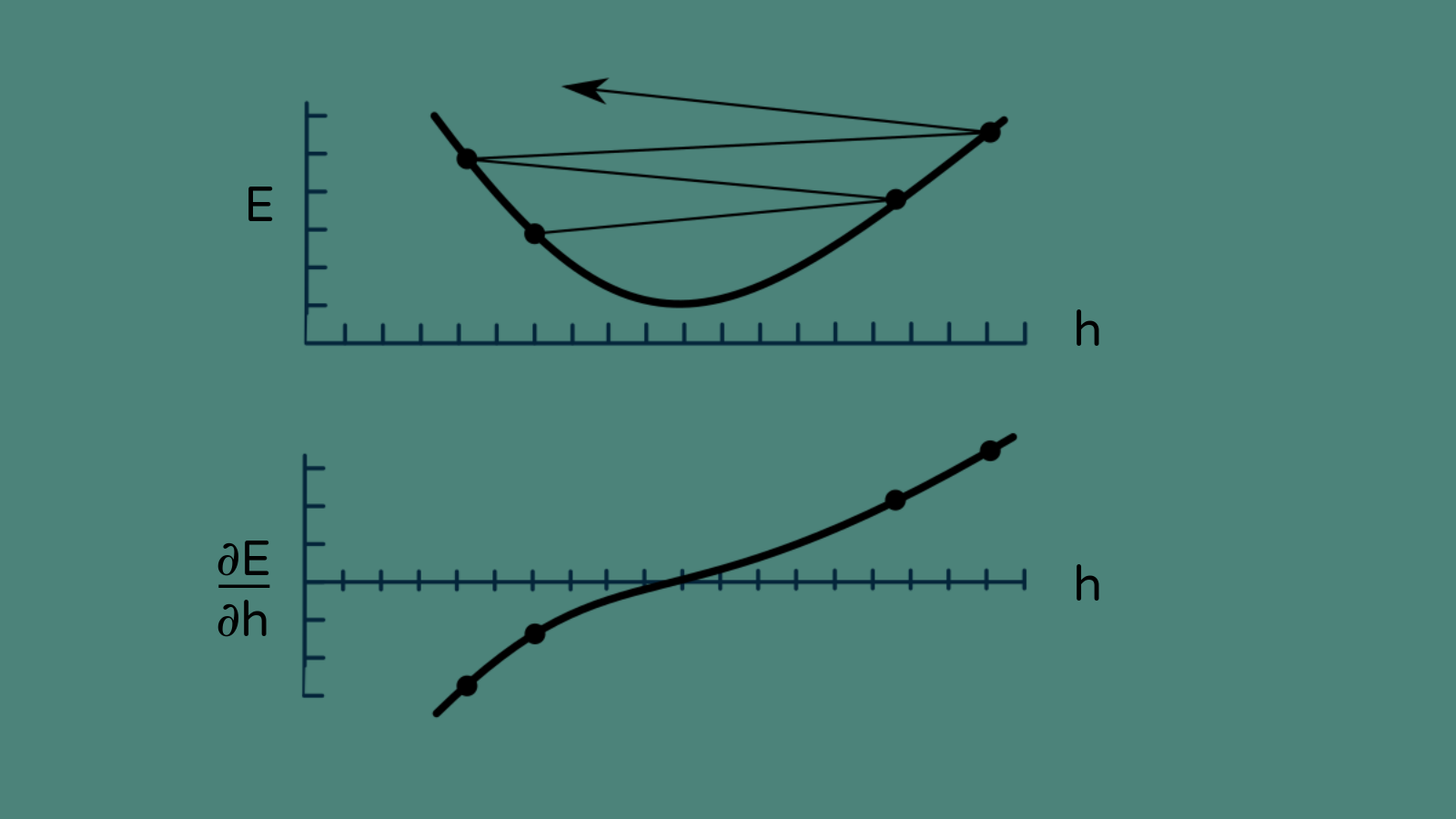
The second reason is that our sensitivities are probably nonlinear. That means that ∂y/∂h, the change in shower flow rate with respect to shower handle position, will be different depending on whether we’re at position h = 2 or at position h = 7. Graphically, the relationship may not be a straight line with a constant slope. It’s probably a curve. The implication of this is that if we make a large adjustment, we are jumping a long way along the curve, but pretending it's a straight line. In all probability we will end up deviating wildly from the curve, and getting an unexpected result.

The third reason is that our sensitivities, remember, are partial derivatives, meaning they also depend on other values. ∂y/∂h might be a larger number if the house flow rate x is high than when the house flow rate is low. And because we are also changing the main valve setting m at the same time, the house flow rate will probably change too. The whole foundation on which we calculated our initial set of sensitivities will shift.

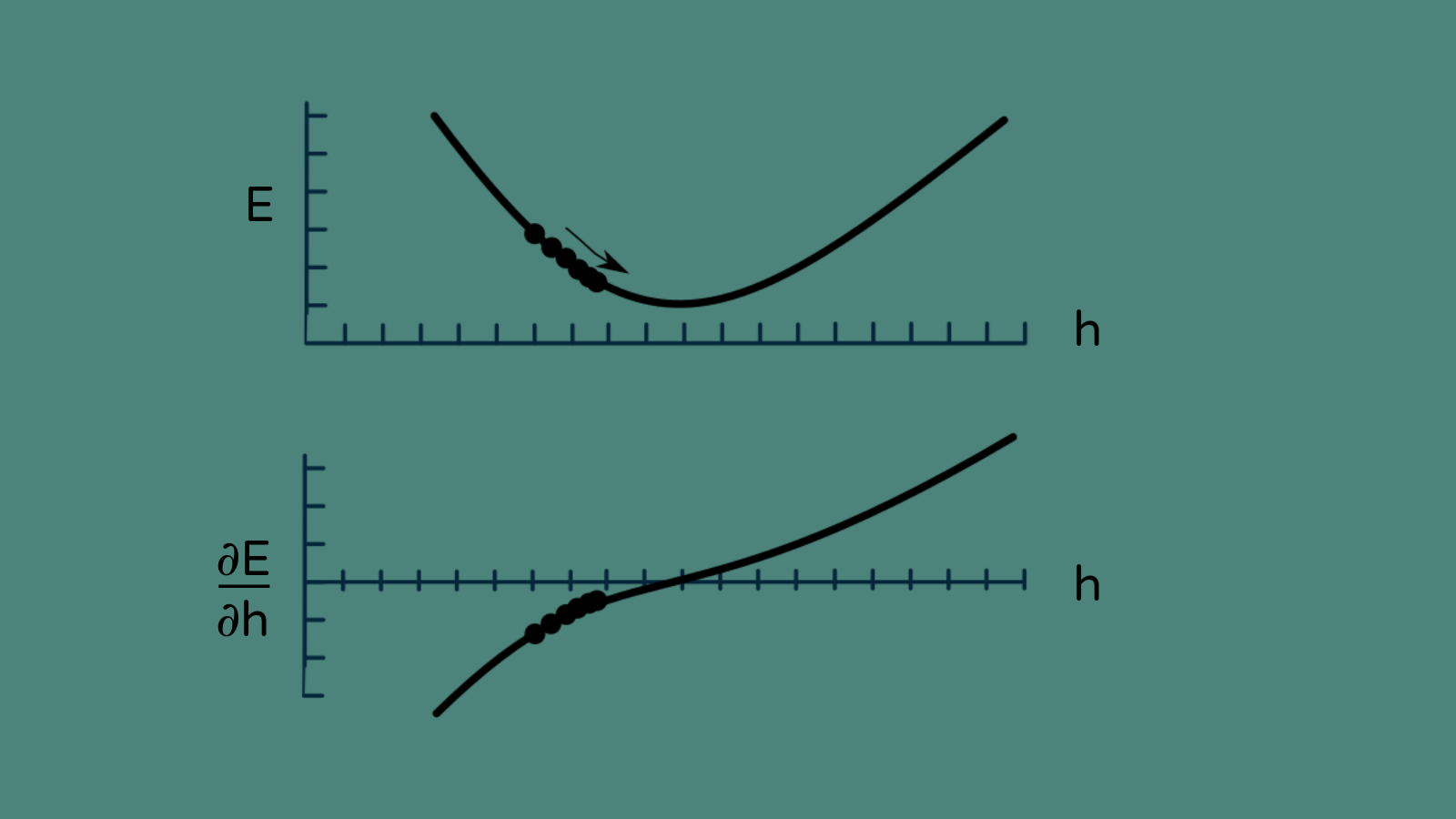
The safest way to handle an uncertain, nonlinear, dynamic situation like this is to take tiny steps. Instead of trying to move the whole distance all at once, move 1/100, or 1/1000, or 1/10,000 of the way. It means that you have to make a lot of steps, but at least your chances of settling into a good answer are much better. This fraction of the distance that we choose to nibble is called the learning rate. Choosing a learning rate that is too large will cause us to bounce around wildly without finding a viable solution. A learning rate that is too small will take an unreasonably long time to reach a solution. The baby steps will just be too tiny. A learning rate of 1/1000 is not a bad place to start, but keep in mind that the ideal learning rate will be different for every problem you try.

Making the first adjustment

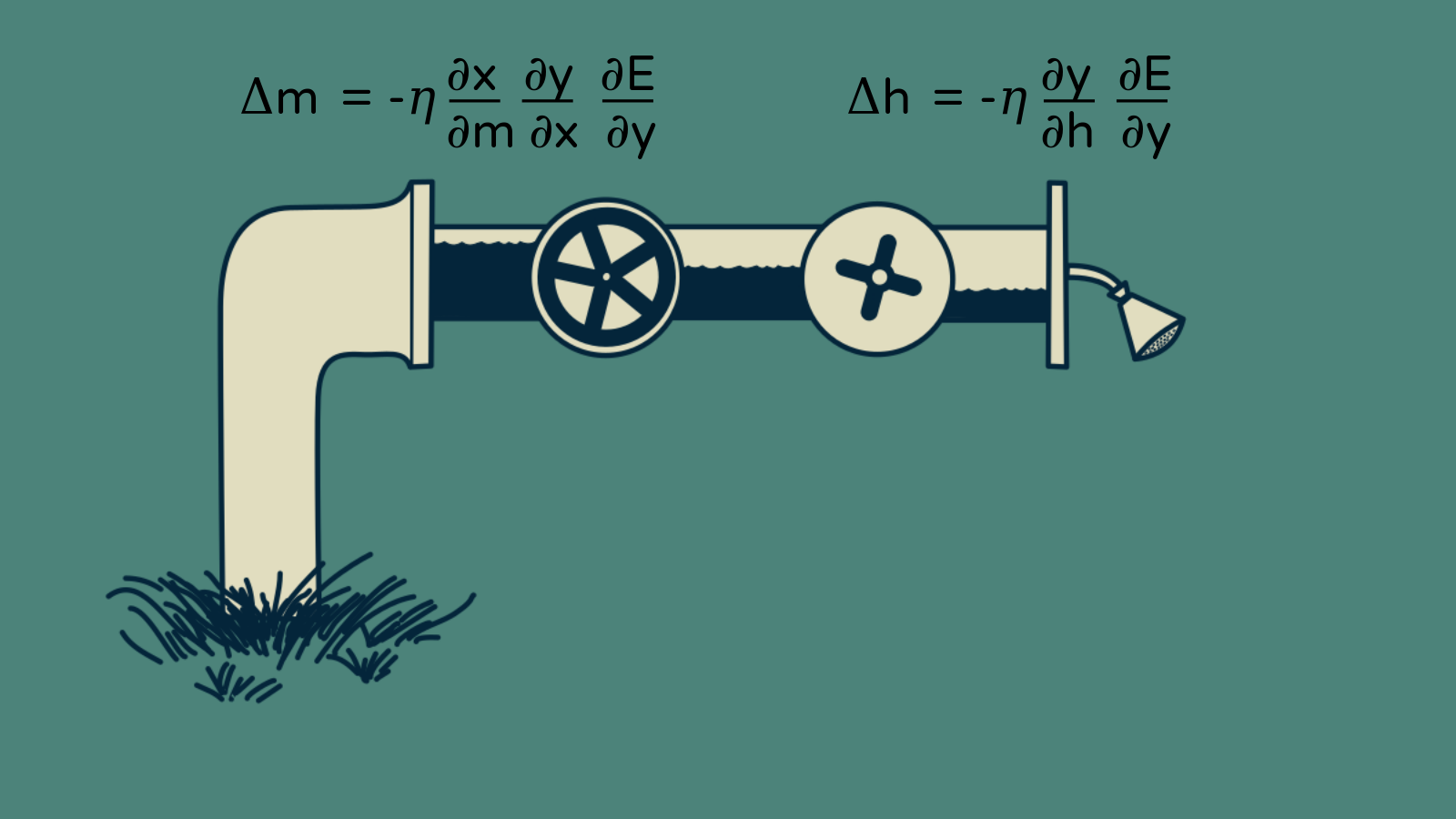
Now we finally know everything we need to adjust our valves and get our shower set up. Each valve adjustment will be proportional to the sensitivity of the error to that valve, and in the opposite direction (we want E to go down, not up). We multiply that by our learning rate, η.

So for our first iteration, our adjustment to the shower handle, Δh1, is −η × ∂E/∂y × ∂y/∂h. Similarly, the change to the main valve, Δm1, is −η × ∂E/∂y × ∂y/∂x × ∂x/∂m.

Congratulations! We have used the chain rule to backpropagate sensitivities through our little network and make small adjustments to the valves. Now we are roughly 100th of the way to a great shower.

The bad news is that all of our sensitivities have now changed. They may have changed a lot. We need to recalculate them.

The good news is that we have everything we need to do that. We made our small changes to the valve settings, Δm₁ and Δh₁, and all we need to do is note the changes in the house flow rate, Δx₁ and the shower flow rate, Δy₁, that resulted from these changes. We can use these to calculate new estimates for the sensitivities in just the same way we did before. This is a computationally cheap way to recalculate our sensitivities.

Now we are really off to the races. All that lacks is to repeat the procedure of making a small change to each valve and updating our sensitivity estimates 100 or 1000 times, until the shower temperature gets close enough to ideal that we don’t care about the difference anymore.

Gradient descent and other learning rate schedules

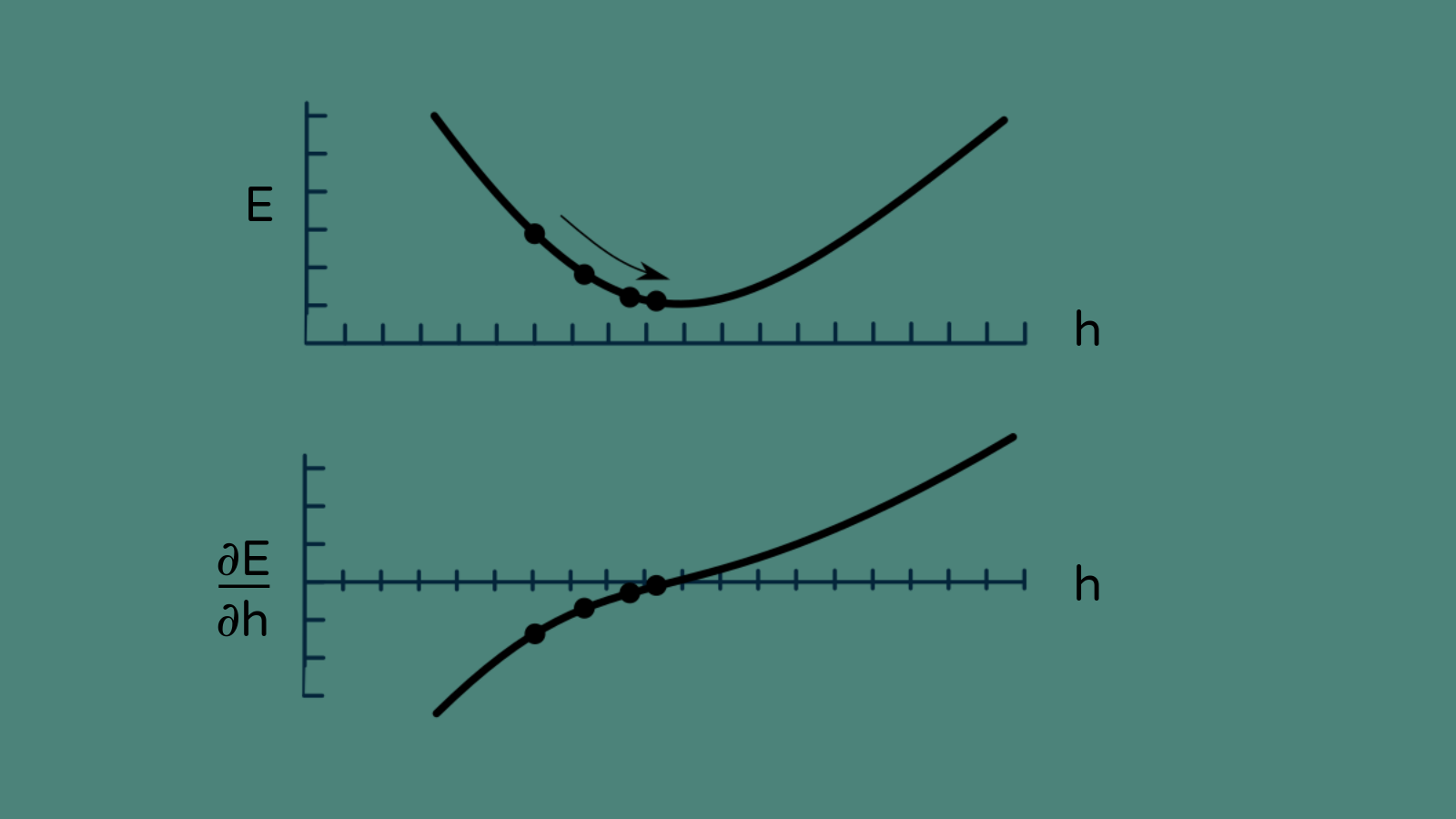
Having a small, fixed learning rate is only one way to make use of our sensitivities. If you imagine our error E as a valley, this approach is analogous to taking a step in the downhill direction. The steeper the hill, the larger the step. This is called gradient descent.

There are other approaches that also use the results of previous steps to to make better guesses about where to step next. They have names like AdaGrad and Momentum and have been shown to work really well. But every single one of them makes use of backpropagation to find the sensitivities of the error to each of the knobs we can adjust.

Backpropagation in the real world

And that’s backpropagation in the world's simplest network.

In our shower example there were just two valves - two knobs to adjust. These were the weights of our little network. In a real neural network there will likely be thousands or millions of these. In our example we just had one hidden layer - the house flow rate. In a real neural network there can be a dozen layers or more. However, the principles of backpropagation are the same:

1. chain sensitivities back through the network,
2. make a small update,
3. observe the effects,
4. update the sensitivities throughout the network,
5. and repeat.

Write your own backpropagation code

Now that you’ve seen how backpropagation works youre ready for the next step - to code it up for yourself. Come join me in the Build a Neural Network Framework course in my End to End Machine Learning school. Together we’ll code up a whole neural network framework in python, start to finish, including backpropagation.

Thanks for stopping by.

Happy building!